Tutorial A.4 — Many copies in one run (better GPU utilization)
Goal: run many non-interacting copies of a single chain in one simulation, so a GPU (which is wasted on one ~100-bead chain) stays busy and you collect N independent trajectories per run for better sampling. Then split the multi-chain trajectory back into per-chain DCDs for normal analysis.
Time: the 10-copy demo finishes in a few seconds on a CPU; the real win is on a GPU.
Prerequisite: Tutorial A.1.
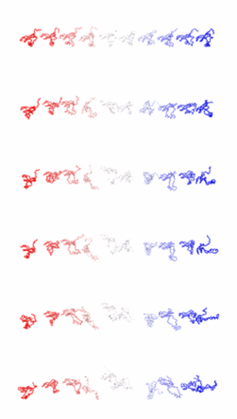
The run — every copy evolves independently, giving 10 trajectories per run to split apart for analysis.
Why do this?
A coarse-grained protein is tiny — P0CX28 is 106 CA beads. A modern GPU can
integrate tens of thousands of particles per step at almost the same wall-clock
cost as a few hundred, so simulating one small chain leaves the device almost
idle. Packing n_copies independent chains into a single System fills the GPU
and turns one run into n_copies trajectories — exactly what you want when a
study needs many trajectories for statistics (folding rates, free-energy
estimates, etc.).
The copies must be truly independent (no chain should feel another). This is guaranteed two ways:
bonded terms (bonds/angles/torsions) and constraints are duplicated within each copy with offset atom indices, and
every
CustomNonbondedForce(the Yukawa electrostatics and the structure-based contacts) is restricted to intra-copy interactions via OpenMMaddInteractionGroup(group_k, group_k).
A direct check confirms the potential is separable: evaluated on the freshly
replicated starting configuration — where every copy is an identical translate of
the single chain — the total potential energy equals exactly N × the
single-chain energy. This is a property of the initial state that verifies no
inter-copy term leaked in; it is not a conserved identity. Once the run starts,
each copy receives independent Langevin forces and diverges, so at later times the
total energy is no longer N × any single chain’s energy — only the strict
independence of the copies is preserved.
Files in this folder
File |
Role |
|---|---|
|
Single-chain input structure (106 residues). |
|
Calibrated single-domain nscale (2.5044), as in Tutorial A.1 (syntax: Domain definition file). |
|
Config; note the |
|
Optional one-line shim to |
|
Optional shim around |
How it works in the run script
Multi-copy support is controlled entirely by n_copies (default 1).
run_simulation.py is a thin shim to the packaged runner topo.mdrun; the
replication itself lives in the shared build step topo.engine.build_system,
which adds one conditional right after building the single-chain model:
cgModel = topo.models.buildCoarseGrainModel(cfg.pdb_file, **cfg.build_kwargs())

if cfg.n_copies > 1:
    system, topology, positions = topo.make_noninteracting_copies(
        cgModel.system, cgModel.topology, cgModel.positions,
        n_copies=cfg.n_copies, shift=cfg.copy_shift * unit.nanometer)
else:
    system, topology, positions = cgModel.system, cgModel.topology, cgModel.positions
# ... everything below runs on (system, topology, positions) unchanged ...
So Tutorials A.1–A.3 and this one use the same runner (topo.mdrun); only
n_copies in md.ini differs.
make_noninteracting_copies is the package primitive that takes the single-chain
model and returns the replicated (system, topology, positions). It wraps
replicate_system_intra_only, replicate_topology and replicate_positions
(all on topo). Copy k is the contiguous atom block [k*n : (k+1)*n].
Step-by-step
1. Set n_copies in md.ini
n_copies = 10          ; independent chains in one run
copy_shift = 5.0       ; nm, x-offset between copies at the start
device = CPU           ; <-- set to GPU on a CUDA machine; that's the point
2. Run
topo-mdrun -f md.ini # or: python -m topo.mdrun -f md.ini
The same standard runner is used as in Tutorials A.1–A.3; because n_copies = 10
its if cfg.n_copies > 1 branch replicates the model via
topo.make_noninteracting_copies. Output goes to the traj/ run folder (DCD +
PSF only, no PDB): traj/traj.dcd (all chains), traj/traj.log, traj/traj.chk,
traj/traj.psf (single-chain topology) and traj/traj_multi.psf
(multi-chain topology, matches the combined DCD).
The in-folder
run_simulation.pyis just a one-line shim (from topo.mdrun import mdrun; mdrun()) kept so the tutorial is self-contained;python run_simulation.py -f md.iniis exactly equivalent.
3. Split into per-chain trajectories
python -m topo.utils.multichain -f traj/traj.dcd -tp traj/traj.psf -o traj --outname traj
This writes traj/traj_{0..9}.dcd — one ordinary single-chain trajectory per
copy (each recentred per frame; pass --no-center to keep raw coordinates). It
streams the combined DCD in chunks so it scales to trajectories too large to fit
in memory. Passing the single-chain PSF with -tp infers n_copies from the
DCD’s atom count (or give -n 10 explicitly). The in-folder split_chains.py is
a thin wrapper around the same routine (topo.split_chains) that reads paths from
md.ini. Load each split trajectory with the single-chain PSF:
import MDAnalysis as mda
u = mda.Universe("traj/traj.psf", "traj/traj_0.dcd")
# RMSD, Q, Rg, ... per independent trajectory
Notes & tips
Pick
n_copiesfor your GPU. Start with 10–50 small chains and increase until the per-step time stops being flat (you’ve saturated the device). Memory is the eventual limit.Independent sampling. Each copy gets different random Langevin forces, so the
n_copiestrajectories are independent samples of the same ensemble — ideal for averaging observables and estimating error bars.copy_shiftonly sets the starting separation; since the chains never interact, its exact value does not affect the physics (it keeps the initial structure tidy and easy to view).No PBC here. With
pbc = nothe chains simply occupy different regions of space. If you enable PBC, make the box large enough to hold all shifted copies.
Performance benchmark
The plot below quantifies exactly this trade-off on a realistic chain — a
360-residue protein — swept over n_copies from 1 to 2048 on five GPUs
(T4, P100, V100, A40, A100), each point averaged over three replicates.
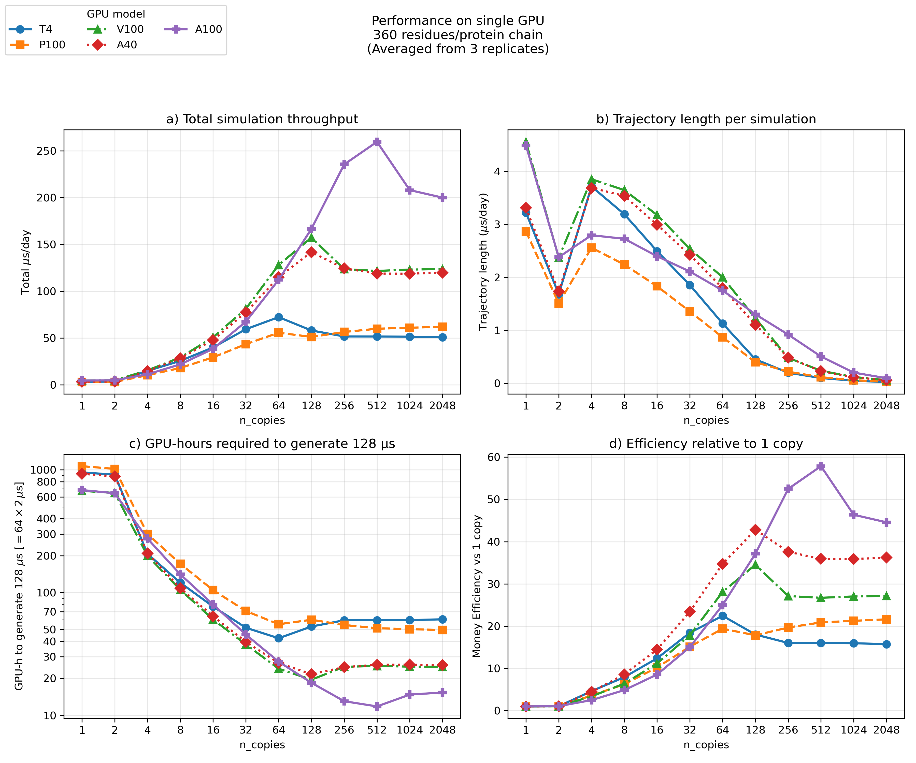
(a) Total throughput — aggregate µs/day summed over all copies — climbs steeply as copies fill the device, then saturates once the GPU becomes compute-bound. Both the height of the plateau and how many copies it takes to reach it are set by the card: the A100 keeps scaling to ~260 µs/day near 512 copies, the V100/A40 level off around 120–155 µs/day, and the older T4/P100 saturate near 50–70 µs/day by ~64 copies.
(b) Per-chain rate — µs/day advanced by any single copy — falls monotonically as the fixed GPU is shared across more chains. This is the price of aggregate throughput: each individual trajectory progresses more slowly in wall-clock time.
(c) GPU-hours for a fixed amount of sampling (here 128 µs) is the practical figure of merit. It drops by more than an order of magnitude from 1 copy to the sweet spot, bottoming out around 128–512 copies before flattening — that minimum is the most cost-effective
n_copiesfor each card.(d) Efficiency vs 1 copy — throughput per copy normalized to the single-copy run — makes the win explicit: up to ~35–58× more sampling per GPU-hour on data-center cards at their optimum.
Reading it for your own runs: pick n_copies near the knee of panel (c)/(d)
for your GPU. Newer, larger cards (A100) keep scaling to several hundred copies;
older or smaller ones (T4, P100) saturate by a few dozen, so pushing past that
buys little. Beyond the optimum, the per-copy rate (b) keeps dropping while total
throughput (a) is already flat — very large n_copies just slows each individual
trajectory for no aggregate gain (and eventually runs into GPU memory limits).
Try next
Switch
device = GPUand compare ns/day forn_copies = 1vs50— the per-copy cost drops sharply once the GPU is filled.Apply the same pattern to the multidomain system from Tutorial A.2.