Disordered / IDR regions

TOPO can mark part (or all) of a chain as an intrinsically disordered region (IDR) — a stretch with no stable fold. A disordered region is declared as an optional disordered: section inside the same domain_def file you already pass through domain_def; there is no separate file, argument, or INI key. This page explains how the model treats a disordered region (the physics) and how you define one (the YAML).

Note

Scope. This is the α-carbon (Cα) model only. The disordered treatment is applied by topo.utils.nonbonded.apply_disorder() at the end of the non-bonded build, and is picked up automatically by isolated-protein simulations, the native-contact (Q) analysis, the nscale optimizer, and continuous synthesis (CSP) — all from the one disordered: section.

The idea in one paragraph

In TOPO the local backbone (3.81 Å bonds, the double-well transferable angle, and the Karanicolas transferable dihedral) is already the disorder-appropriate, non-Gō backbone for every residue — see The TOPO model: theory and force field. What makes a residue in a folded domain folded is therefore only its native (Gō) contacts. Marking a region disordered means: remove its native contacts and replace them with a weak, non-specific attraction, while keeping self-avoidance. Bonds, angles, dihedrals and electrostatics are untouched; what changes is the contact term, and only for pairs that touch a disordered residue — those move to a second CustomNonbondedForce with a different functional form (below), leaving folded–folded pairs on the Gō 12-10-6 exactly as before.

How a disordered region is treated in the model

Every residue pair falls into exactly one of three classes, decided by how many of its two residues are in the disorder mask. The class fixes the pair’s well depth, its well position, and — unlike a purely folded build — which of two forces evaluates it:

Pair class	Force	Native (Gō) contacts	Well depth \(\varepsilon_{ij}\)	Well position \(R_{ij}\)
folded–folded (neither residue in the mask)	12-10-6 (Structure-based contacts)	kept (Gō)	unchanged — H-bond + backbone–sidechain + scaled sidechain–sidechain, else the non-native floor	native Cα distance, else the Karanicolas–Brooks (K–B) sum rule
IDR–IDR (both residues in the mask)	Ashbaugh–Hatch 12-6	removed	\(\max\!\bigl(\varepsilon_\mathrm{NN},\ s_\mathrm{IDR}\,\varepsilon_\mathrm{BT}\bigr)\) (defined below)	\(R_\mathrm{min}/2 + R_\mathrm{min}/2\) (sum rule)
folded–IDR (exactly one residue in the mask)	Ashbaugh–Hatch 12-6	removed	\(\max\!\bigl(\varepsilon_\mathrm{NN},\ s_\mathrm{IDR}\,\varepsilon_\mathrm{BT}\bigr)\) — the same rule as IDR–IDR	\(R_\mathrm{min}/2 + R_\mathrm{min}/2\) (sum rule)

The two forces carry disjoint interaction groups — the 12-10-6 gets {folded} × {folded}, the Ashbaugh–Hatch force gets {idr} × {idr} and {idr} × {folded} — so every pair is evaluated exactly once. (OpenMM sums forces independently and takes the union of a force’s interaction groups, so a pair admitted to both would silently receive both potentials, added together, with no error raised. Each force’s groups are therefore set once, by the code that creates it, and never widened afterwards.)

Above, \(s_\mathrm{IDR}\) is the idr_scale knob, \(\varepsilon_\mathrm{NN}\) is the non-native floor (\(1.32\times10^{-4}\) kcal/mol), and \(\varepsilon_\mathrm{BT}(i,j)\) is the sidechain–sidechain BT interaction energy for the two residue types — the same per-pair energy the model uses for native SS contacts, namely

\[\varepsilon_\mathrm{BT}(i,j) \;=\; 4.184 \cdot \bigl|\,\mathrm{raw}(i,j) - 0.6\,\bigr| \quad\text{[kJ/mol]},\]

i.e. the raw bt_potential.csv value shifted by the 0.6 kcal/mol reference, made positive with \(|\cdot|\), and converted kcal→kJ (this is exactly topo.utils.nonbonded.get_ss_interaction_energy()) — not the bare CSV number.

Depth — one channel, one rule. Every non-local pair that touches a disordered residue gets

\[\varepsilon_{ij}^\mathrm{IDR} \;=\; \max\!\bigl(\varepsilon_\mathrm{NN},\; s_\mathrm{IDR}\,\varepsilon_\mathrm{BT}(i,j)\bigr)\]

\(\varepsilon_\mathrm{BT}(i,j)\) carries the sequence dependence. It is non-specific in coverage (it acts on every non-local IDR–IDR pair, not just would-be native contacts) but chemically heterogeneous in depth — the BT energy varies by residue-pair type, so a hydrophobic pair attracts more strongly than a polar one. idr_scale (\(s_\mathrm{IDR}\)) scales it, and is the single solvent-quality dial: raising it lowers the scaling exponent \(\nu\).

The same rule applies to folded–IDR cross pairs: the depth is a property of the two residue types, not of which region each one sits in. A hydrophobic IDR bead near a hydrophobic surface bead attracts for exactly the reason it would inside the IDR, so there is no branch on region anywhere in the depth expression. This is also what dedicated IDP force fields do — HPS/Dignon draw no folded/disordered distinction at all. The practical consequence is that a disordered tail can adsorb onto its own folded core rather than only sampling free solution.

Warning

The cross-pair depth is an extrapolation of the calibration, not a result of it. idr_scale = 0.10 was fitted on fully-IDP chains (Validation against SAXS R_g), where every pair is IDR–IDR — folded–IDR pairs never entered the benchmark. Applying the same scale across the boundary is a modelling choice the SAXS data cannot confirm. If a tail in your system collapses onto its domain more than you can justify, that is the parameter to question first; and if you want the tail to behave as a purely entropic linker, idr_scale: 0 still gives excluded volume only.

Physically this is a weak, non-fold-encoding attraction — a collapsing self-avoiding chain, not a Gō fold. The \(\max(\varepsilon_\mathrm{NN}, \cdot)\) floor keeps a nominal depth even at idr_scale = 0 (and for the handful of pairs whose \(\varepsilon_\mathrm{BT}\approx 0\)); the excluded volume itself comes from eps_ev_kj, independently, as the next section explains.

The IDR functional form — and why it is not the 12-10-6

With \(L(r) = 4\bigl[(\sigma/r)^{12} - (\sigma/r)^{6}\bigr]\) and \(\sigma = 2^{-1/6} R_{ij}\), an IDR-involving pair is evaluated by an Ashbaugh–Hatch split:

\[\begin{split}U_{ij}(r) = \begin{cases} \varepsilon_\mathrm{EV}\, L(r) + (\varepsilon_\mathrm{EV} - \varepsilon_{ij}), & r \le R_{ij}\\ \varepsilon_{ij}\, L(r), & r > R_{ij} \end{cases}\end{split}\]

The minimum sits at \(r = R_{ij}\) with depth exactly \(-\varepsilon_{ij}\) for any \(\varepsilon_\mathrm{EV}\), and the join is \(C^1\). So \(\varepsilon_\mathrm{EV}\) (eps_ev_kj) sets the repulsive core and \(\varepsilon_{ij}\) sets the well depth, independently — the whole point of the form.

The Gō 12-10-6 cannot express this, for two separate reasons. Both matter; fixing either alone is not enough.

1. One \(\varepsilon\) scales both the wall and the well. In \(U = \varepsilon\,[13(R/r)^{12} - 18(R/r)^{10} + 4(R/r)^{6}]\) the same \(\varepsilon\) multiplies the repulsive \(r^{-12}\) term and the attractive well, so there is no way to ask for “more attraction at the same bead size”. Measuring the core as the radius where \(U = +k_BT\), switching on any attraction moves it from 0.58 R to ~0.91 R — a 56 % increase in radius, ~3.7× in excluded volume — to buy a well shallower than \(k_BT\). The excluded-volume gain dominates and the chain expands when attraction is added. Under the Ashbaugh–Hatch split the core moves only 0.846 R → 0.819 R (3.2 %) as \(\varepsilon_{ij}\) runs 0 → 2 kJ/mol, and that residual runs the benign way — more attraction slightly softens the core.

2. The 12-10-6 carries a desolvation barrier. Its coefficients \((13, -18, +4)\) place a repulsive bump beyond the well: the shape function crosses zero at \(1.25 R\) and peaks at \(1.45 R\) at \(+0.143\,\varepsilon\), so a pair must climb \(0.143\,\varepsilon\) before it can reach the well. That barrier is deliberate and physically right for a native contact — forming one requires expelling the solvent between two residues, a real free-energy barrier, and it is what gives Gō models their two-state contact kinetics. Between two disordered residues there is no native contact and no desolvation event to represent. Worse, sitting at larger \(r\) it carries more \(4\pi r^2\) weight in the second virial coefficient \(B_2 = -\tfrac12\int (e^{-U/k_BT} - 1)\,4\pi r^2\,dr\) than the well does, so it holds the θ point (\(B_2 = 0\)) at 1.94 \(k_BT\) where a 12-6 puts it at 0.35 \(k_BT\):

\(\varepsilon_\mathrm{att}\) (kJ/mol)	\(B_2/\mathrm{hs}\) — 12-10-6 split	\(B_2/\mathrm{hs}\) — 12-6 Ashbaugh–Hatch
0.0	0.832	0.744
1.0	0.967	−0.109
2.0	0.993	−1.169
3.0	0.869	−2.516
θ point (\(B_2 = 0\))	4.84 kJ/mol (1.94 \(k_BT\) )	0.88 kJ/mol (0.35 \(k_BT\) )

With the barrier, \(B_2\) rises up to \(\varepsilon_\mathrm{att} \approx 1.5\) — adding attraction makes the chain more swollen. Without it, \(B_2\) falls monotonically from the first increment, which the BT table reaches at \(s_\mathrm{IDR} \approx 0.32\).

This prediction was tested, and it is directional: under the coupled 12-10-6, \(\nu\) rose with idr_scale (0.605 → 0.723 across 0 → 1); under the Ashbaugh–Hatch 12-6 it falls (0.637 → 0.276 across 0 → 0.30), sweeping through the experimental 0.551 and out the other side into collapse. Same benchmark, same proteins, opposite sign — the functional form, not the parameter value, was the defect.

A plain 12-6 with a single \(\varepsilon\) would re-introduce defect 1. The Ashbaugh–Hatch construction splits the potential at its minimum, holding the repulsive branch fixed and scaling only the attractive branch, which is exactly the separation required — and it yields a clean WCA limit at \(\varepsilon_{ij} = 0\): a purely repulsive bead of physical size, so “no attraction” and “no excluded volume” finally become independent statements. This is the standard form in dedicated IDP force fields (HPS/Dignon, Ashbaugh–Hatch), and it is why the hydropathy parameter behaves as a solvent-quality dial there.

Folded–folded pairs keep the 12-10-6, barrier and all, because there the barrier is doing the job it was designed for. The change is scoped precisely to pairs where a native contact does not exist.

Note

The depth carries no nscale factor. The IDR depth uses the \(\varepsilon_\mathrm{BT}\) matrix above (unscaled by any domain factor), not the domain-scaled sidechain energy. In TOPO nscale is the per-domain folding-stability ladder (Why stability must be calibrated); an IDR has no fold and no stability target, so it does not inherit a ladder value (effectively nscale = 1 for IDR pairs).

So at idr_scale = 1.0 an IDR–IDR pair would get a sequence-dependent attraction equal to the unscaled (nscale = 1) sidechain–sidechain interaction energy that the same pair of residue types carries as a native contact — \(\langle\varepsilon_\mathrm{BT}\rangle \approx 2.36\) kJ/mol. That is far past the θ point; the calibrated default is idr_scale = 0.10, i.e. ~10 % of a native sidechain contact. Read it against the raw SS energy, not against a folded domain’s contacts: a real domain additionally scales its SS contacts by its own nscale (typically > 1), so relative to that the IDR attraction is weaker still.

Position — the excluded-volume radius. The collision radius is a property of the residue. For a residue in an IDR region the structure-derived K–B radius is meaningless (its input coordinates do not define a fold), so those residues take the transferable per-AA \(R_\mathrm{min}/2\) from the parameter table. Residues in folded domains keep their K–B \(R_\mathrm{min}/2\) unchanged. Both populations therefore carry the same quantity, and every pair combines by the plain sum rule:

\[R_{ij} = R_\mathrm{min}/2_i + R_\mathrm{min}/2_j \qquad\text{for every pair class, cross pairs included.}\]

Note

The radius is an \(R_\mathrm{min}/2\) , not a σ-radius. The R slot of both the 12-10-6 and the Ashbaugh–Hatch form is an \(R_\mathrm{min}\), and calculate_rmin_2_values() produces the same quantity for folded beads — so no \(2^{1/6}\) division is applied when populating the per-residue radius array. The conversion lives inside the IDR force’s own expression, where \(\sigma = 2^{-1/6} R_{ij}\) recovers the van der Waals sum. That is also why the σ values are directly comparable to a published IDP force field: \(\sigma = (R_\mathrm{min}/2_i + R_\mathrm{min}/2_j)/2^{1/6}\) reproduces the HPS per-residue σ to a mean −0.1 % (max 1.5 %, glycine exact), which is what makes eps_ev_kj = 0.8368 (the HPS value) transferable here by construction.

A residue in a folded domain keeps its native radius even when it meets a residue in an IDR region — it is not shrunk in cross pairs. Because the override is applied to the per-residue radius array, the same radius reaches both the intra-chain and (for synthesis) the nascent↔ribosome excluded-volume channels — they cannot disagree. No new parameter file is shipped.

What does not change. Bonds, angles, dihedrals, and Yukawa electrostatics are untouched (the global transferable backbone is already the disordered-appropriate choice). A run with no disordered: section builds the single unrestricted 12-10-6 exactly as before and is byte-for-byte identical; even with a section, folded–folded well positions and depths, and the K–B radius of every residue in a folded domain, are unchanged to floating-point equality.

Warning

Declaring an IDR deletes cross-boundary native contacts. Every native contact with one end in the disordered region is removed — intended (a disordered residue’s crystal contacts are artifacts) but not free. For the 4c5c tutorial system with residues 1–40 disordered, 88 of 819 contacts go and 34 folded residues lose at least one contact, so the folded remainder is a less stabilized fold than the full Gō model. The build prints the count. This is also why you must run the nscale optimizer on the domain_def that already contains the disordered: section (see below).

Defining a disordered region in domain.yaml

Add a disordered: block to the domain_def file. All three top-level sections (intra_domains, inter_domains, disordered) are optional; only n_residues is required.

Important

Deciding which residues are disordered. Choosing the disordered residues is your responsibility — TOPO applies exactly the set you list in residues: and makes no attempt to detect disorder itself. The definition of an IDR is model-dependent, so the ranges you commit to are a modeling choice you should be able to justify. The following are common sources to inform that decision (not automatic assignments):

• MobiDB (https://mobidb.org/) — a database of protein disorder and mobility that aggregates curated and predicted intrinsically disordered regions. Look up your protein by its UniProt accession to see candidate disordered ranges.

• AlphaFold pLDDT < 70 — residues whose AlphaFold per-residue confidence (pLDDT) falls below 70 are a widely used proxy for disorder: low-confidence stretches correspond closely to intrinsically disordered regions. This is the threshold used to define IDRs at proteome scale in Tesei et al. [Tesei2024]. The pLDDT is stored in the B-factor column of the AlphaFold model.

Both report 1-based residue numbers. Treat them as evidence, reconcile them against your own knowledge of the system, and then enter the ranges you decide on into the residues: list below.

n_residues: 283

# --- domain scaling of native side-chain contacts (optional, unchanged) ---
intra_domains:
  A: { residues: [25-149],  nscale: 1.0 }
  B: { residues: [150-283], nscale: 1.0 }
inter_domains:
  A-B: 0.5

# --- disordered / IDR region (optional) ---
disordered:
  residues: [1-24, 150-165]   # native contacts removed for these residues
  idr_scale: 0.10             # OPTIONAL, well depth; defaults to 0.10
  eps_ev_kj: 0.8368           # OPTIONAL, repulsive core (kJ/mol); defaults to 0.8368

The residue-list syntax is exactly the one used everywhere else in the file: inclusive ranges as strings ("1-24"), bare integers, or a mix ([1, 2, "5-10", 150-165]). Numbering is 1-based and matches the input PDB.

Field reference

Key	Required?	Type (default)	Meaning / allowed values
disordered	no	mapping (absent)	Presence of this block turns on the IDR treatment. Omit it entirely for a fully-folded protein (then the run is byte-identical to before).
disordered.residues	yes (if the block is present)	list (—)	Residues to mark disordered. Same syntax as a domain’s residues: ranges ("1-24", inclusive), bare integers, or a mix. Their native contacts are removed.
disordered.idr_scale	no	float (0.10)	The scale \(s_\mathrm{IDR}\) on the sequence-dependent BT channel — i.e. the IDR–IDR well depth, and the only compaction knob. Defaults to 0.10, the calibrated value (Validation against SAXS R_g). Raise it to compact, lower it to expand; 0 gives a pure self-avoiding chain. The θ point is at \(\approx 0.32\) — above that the chain collapses, so treat a value much beyond ~0.3 as suspect. It sets the depth for folded–IDR cross pairs too.
disordered.eps_ev_kj	no	float (0.8368)	The repulsive-core strength \(\varepsilon_\mathrm{EV}\) (kJ/mol) of the Ashbaugh–Hatch force, independent of the well depth. Defaults to 0.8368 (0.2 kcal/mol, the HPS/Dignon value). It is a weak handle on bead size — the core goes as \(\varepsilon_\mathrm{EV}^{1/12}\), so a 100× change moves the bead only ~46 %. If bead size must change, change the radius table.

Overlap with a domain is allowed — disorder wins

A disordered: range may overlap an intra_domains range. The disorder transform runs after the whole folded build (including domain scaling), so for any pair touching a disordered residue the domain nscale is computed and then discarded — the pair is governed entirely by the disorder rules. In other words: if either residue of a pair is disordered, disorder governs it, no matter which domains the two residues belong to.

This makes overlap a convenience — define a domain broadly and carve a disordered loop out of it without splitting the domain:

n_residues: 100
intra_domains:
  A: { residues: [1-100], nscale: 1.6871 }   # one domain over the whole chain ...
disordered:
  residues: [40-50]                           # ... with a disordered loop carved out

Here residues 40–50 are disordered (their nscale has no effect); the rest of domain A folds as one unit with a hole, still joined across the loop by its 40↔ folded and 50↔ folded backbone bonds and by the retained 1–39 ↔ 51–100 contacts. The reader prints an info line listing any overlapping residues, so an accidental double-listing is visible (it is not an error — overlap is legal).

Tuning the compaction

• The default is calibrated (idr_scale = 0.10) — use it unless you have a specific reason not to. It was fit against SAXS \(R_g\) for 18 disordered proteins (Validation against SAXS R_g). A chain with no attraction at all systematically over-expands most IDPs: SAXS/smFRET place them at scaling exponent \(\nu \approx 0.5\text{–}0.55\), versus \(\nu \approx 0.588\) for a self-avoiding walk. The non-specific attraction reweights the same broad, flexible ensemble toward the observed compaction without locking in a fold. Because TOPO’s Debye–Hückel electrostatics are always on (a repulsive term for charged chains), the balanced physical picture is repulsion balanced by weak attraction.

• To tune compaction, move idr_scale. It is now a true solvent-quality dial: raising it lowers \(\nu\), as attraction physically should. Do not reach for eps_ev_kj — that sets bead size, not solvent quality, and is a very weak handle on size at that.

• Values above ~0.32 are past the θ point and give a collapsed globule. If you have carried an idr_scale over from an older domain_def (the previous default was 1.0), delete the key and take the new default, or set 0.10. A value someone fitted against the old coupled 12-10-6 has no meaning under this force and must be re-fitted.

• Self-avoiding is the better call for: a disordered linker whose role is reach / entropic tethering (compaction is not the observable); a strongly charged, highly expanded IDP that genuinely approaches self-avoiding-walk statistics; or a deliberately minimal, assumption-free reference ensemble. Set idr_scale: 0 — and note this now gives a self-avoiding chain of physical bead size, since eps_ev_kj still sets the core.

• Re-calibrate when you can. If you have SAXS/smFRET \(R_g\) or \(\nu\) for your system, treat idr_scale as the fit parameter.

Validation against SAXS \(R_g\)

The default was calibrated and validated on a benchmark of 24 proteins (24–273 residues) with published SAXS radii of gyration, of which 18 are used for calibration and 6 are reported as a control (see the split below). Each protein was simulated as a fully-IDP chain (residues: [1-N]) for 90 ns of Langevin dynamics at 300 K from an expanded-coil start, discarding the first 15 ns; the reported \(R_g\) is the mass-weighted ensemble average \(\sqrt{\langle R_g^2\rangle}\) over the remaining 75 ns.

Important

The 18/6 split is a judgement, not a datum. Six of the 24 — CspTm, R15, R17, hCyp, Protein-L, sNase — are foldable globular proteins whose published \(R_g\) is a folded-state value. Simulating them as fully disordered chains and comparing to that number measures nothing about the IDR model, so they are excluded from the calibration. That classification is made by protein identity and is not recorded in the dataset; if it is wrong for any of them the fitted idr_scale shifts (including all 24 moved the optimum measurably). The split, its members and its rationale are stated here so the choice is visible and can be revisited, and the 6 are always reported as a control rather than dropped silently.

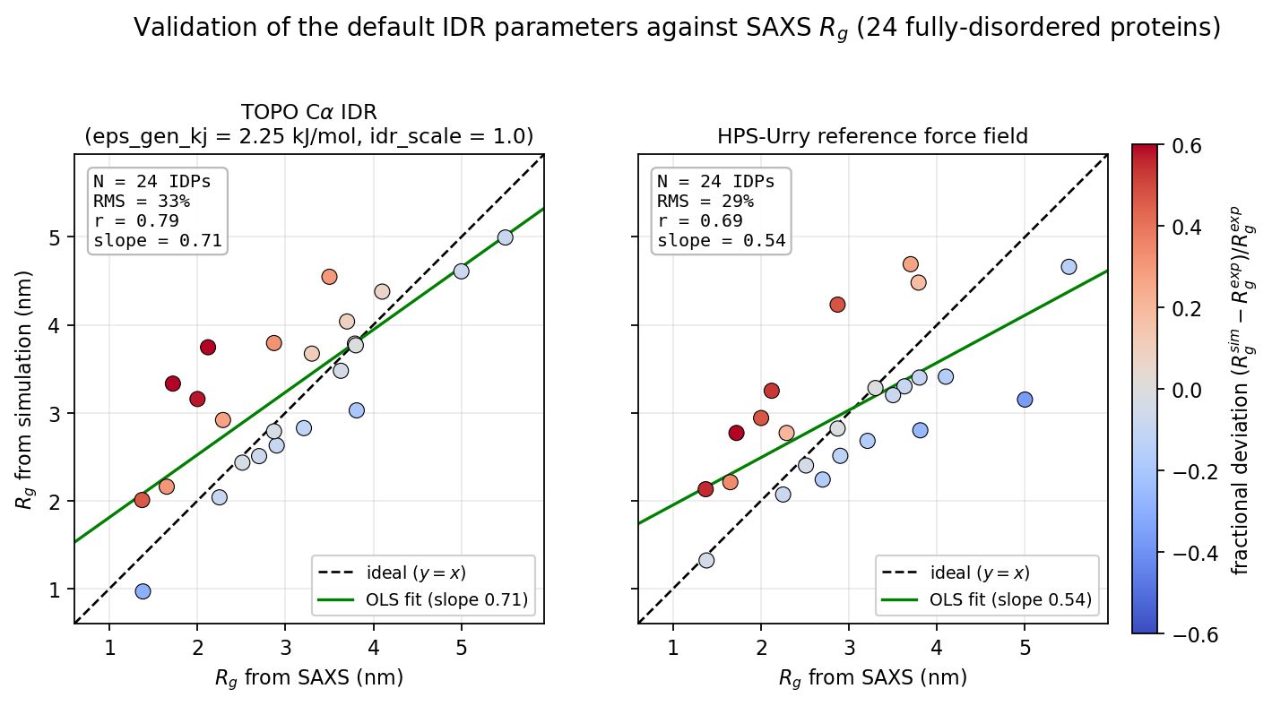
Left: TOPO’s Cα IDR model at the calibrated defaults idr_scale = 0.10, eps_ev_kj = 0.8368 kJ/mol. Right: the HPS-Urry force field on the same 18 proteins, as an external reference point. Dashed line is \(y = x\); green is the ordinary-least-squares fit; point colour is the fractional deviation. TOPO tracks \(y = x\) across the range, while HPS-Urry runs systematically compact (blue) and flattens at the expanded end — the slope difference, 0.81 against 0.68.

Fitting the scaling law \(R_g = R_0 N^{\nu}\) over the 18 IDPs, at idr_scale = 0.10 and eps_ev_kj = 0.8368:

Model	\(\nu\)	\(R_0\)	RMS	Pearson r	OLS slope
TOPO Cα IDR (this model)	0.566	0.223	12.0 %	0.89	0.81
HPS-Urry (reference)	0.490	0.301	19.7 %	0.70	0.68
experiment	0.551	0.244	—	—	—

RMS is the root-mean-square fractional deviation \(\sqrt{\tfrac{1}{N}\sum_i \bigl((R_g^\mathrm{sim} - R_g^\mathrm{exp})/ R_g^\mathrm{exp}\bigr)^2}\).

The headline result is that \(\nu\) is tunable and on target: idr_scale acts as a true solvent-quality dial, sweeping \(\nu\) from 0.637 at idr_scale = 0 down through the experimental 0.551 and into collapse (0.276 at idr_scale = 0.30), so the calibrated 0.10 lands on 0.566. A 3-seed confirmation at idr_scale = 0.12 gives \(\nu = 0.559 \pm 0.009\). Against HPS-Urry on the same 18 proteins, TOPO gives a closer exponent, a lower RMS, a higher rank-correlation, and a slope nearer 1 (less compression of the range between compact and expanded chains).

Warning

Read the RMS against the right bar. 12.0 % is not evidence that the model captures sequence-specific differences. The power law is fitted to the same data and still leaves a 9.5 % residual, so a bare \(R_g = 0.244\, N^{0.551}\) — chain length and nothing else — already explains almost all of it. The model does not yet beat chain length alone. Concretely: three chains at \(N = 185\) span 36 % in experiment and 7 % in the model, in the wrong rank order. Closing that gap is a separate problem, believed to lie in the bonded terms or in charge patterning rather than in the contact channel. Use the model for the ensemble dimensions of a disordered region; do not use it to rank two IDPs of similar length against each other.

Note

folded ↔ IDR attraction is on, and it is the same knob. A residue in a folded domain and a residue in an IDR region interact through the same \(\max(\varepsilon_\mathrm{NN}, s_\mathrm{IDR}\varepsilon_\mathrm{BT})\) depth as two IDR residues — transient, non-specific (“fuzzy”) IDR–domain association is therefore an active part of the model, not a future extension. What those pairs never get back is a native contact: any Gō contact crossing the boundary was deleted with the disorder declaration, so the attraction is sequence-weighted and non-specific, never fold-encoding. To switch it off, set idr_scale: 0 — which switches off the IDR–IDR attraction too, since it is one knob.

Note

Starting coordinates do not matter. The equilibrium IDR ensemble is set by the potential (no native contacts + flexible backbone + the IDR attraction idr_scale), not by the input geometry. With its native contacts removed, a region initialized from a folded structure relaxes toward the disordered ensemble; discard the initial relaxation in analysis as you would for any MD run. You do not need to pre-build an extended-chain PDB for the disordered part.

Effect on native-contact analysis (Q) and the nscale optimizer

The IDR mask reaches both of TOPO’s native-contact definitions so that they stay consistent with the energy function:

• Q analysis (Native-contact analysis (the Q score), topo.analysis.native_contacts.build_native_contacts()): any native contact touching a disordered residue is dropped from every Q series (Q_protein, each Q_domain, and interfaces). If it were kept, those never-forming contacts would sit permanently in the denominator and deflate Q. The Q driver reads the same disordered: section from the domain_def you already pass with -d/--domain.

• Effective domain membership = domain − disordered. A residue listed in both a domain and disordered: no longer contributes to that domain’s Q (nor to any interface Q) — mirroring “disorder wins” on the energy side.

• The nscale optimizer (Why stability must be calibrated) optimizes only the folded domains and their interfaces; it does not optimize the disordered region. The IDR is present in every round’s simulation (each round builds its energy through apply_disorder, so the disorder is always active), but it is not a scoring unit and never enters the convergence check — the optimizer makes no attempt to stabilize it. In this it behaves like the auto-created X domain (Domain definition file (domain.yaml)): present in the run at a fixed treatment, but left out of the optimization. Disordered residues are governed by idr_scale and are never assigned an nscale. The masked Q keeps the IDR’s (never-forming) contacts out of each folded domain’s stability score so they cannot deflate it.

Important

Optimize with the IDR present. Because masking a region removes any native contacts it made with a domain, the domain is genuinely less stable when the IDR is present. Always run the optimizer on the domain_def that already contains the disordered: section — do not calibrate on the fully-folded structure and then add disorder afterward.

Continuous synthesis (CSP)

Continuous synthesis honours a disordered: section with no extra configuration: it already threads domain_def into the contact build, and the disorder mask is sliced to the emerged chain at each length (particle i is native residue i+1, so a residue is emerged iff its index is < L). While the emerged chain is still inside a disordered N-terminal prefix the 12-10-6’s interaction group is empty and contributes zero; once folded residues emerge, the Ashbaugh–Hatch force carries both {idr}×{idr} and {idr}×{folded} groups. Because the per-residue radius array is what CSP feeds to both the nascent↔nascent pair matrix and the nascent↔ribosome excluded volume, an IDR nascent bead meets the ribosome with the correct per-AA radius on both sides. With no disordered: section a CSP contact build is byte-identical to before.

Note

The nascent↔ribosome interaction stays a 12-10-6 for every nascent bead, disordered or not, at the unchanged RIBO_NC_EPS_KJ. It is a separate force created by topo.csp.ribosome.append_ribosome(), so this holds structurally — there is no if disordered branch anywhere in that path — and the validated 4c5c reproduction is preserved. The consequence is that a disordered bead is on a different footing toward the ribosome than toward the rest of the chain. That is deliberate: the two are different physics, and the nascent↔ribosome parameters are O’Brien’s, calibrated as a set.

Edge case — a fully disordered protein (IDP)

If every residue is disordered, list them all and omit intra_domains:

n_residues: 92
disordered:
  residues: [1-92]
  # idr_scale / eps_ev_kj omitted -> the calibrated defaults (0.10, 0.8368 kJ/mol)

This fully-IDP case is exactly the configuration the defaults were validated on (Validation against SAXS R_g). The energy build runs normally and is then fully overwritten to IDR–IDR everywhere (finite radii, no native contacts) — a valid collapsing (or, with both knobs at 0, self-avoiding) homopolymer-like chain. The Q analysis returns an empty contact list (Q = NaN, not a crash), and the nscale optimizer detects that there are no foldable contacts and exits cleanly with a “nothing to optimize” message rather than reporting a vacuous convergence (there is genuinely no nscale to tune).

Common pitfalls

• A stale idr_scale from an older domain_def is legal YAML and parses without complaint. The previous default was 1.0, which under this force is ~3× past the θ point and gives a collapsed globule. Delete the key and take the new default, or set 0.10.

• ``idr_scale: 0`` is not “no interaction”. It removes the attraction but keeps the excluded-volume core set by eps_ev_kj, so IDR pairs still cannot interpenetrate. It is a self-avoiding chain of physical thickness, not a ghost chain. (Under the previous coupled form the “zero attraction” limit really was nearly a ghost chain — the bead was thin because it had no energy. That is the coupling this change removed.)

• Numbering must match the structure. Disordered residues use the same 1-based PDB numbering as the domains; a wrong number silently disorders the wrong residue.

• Overlap is silent-but-logged. A residue accidentally left in both a domain and disordered: becomes disordered (disorder wins). The reader prints an info line naming the overlap — check it if a domain seems weaker than expected.

• Single chain only. disordered: is one flat residue set for the system; there is no per-chain qualifier yet.

• YAML indentation — as with the rest of the file, use spaces (never tabs) and put a space after every colon. See YAML syntax in 60 seconds on the Domain definition file (domain.yaml) page.

References

[Tesei2024]

Tesei, G. et al. Conformational ensembles of the human intrinsically disordered proteome. Nature 626, 897–904 (2024). https://doi.org/10.1038/s41586-023-07004-5