Tutorial 1 — Single-domain quickstart¶

Goal: run your first TOPO simulation end-to-end and understand the inputs and outputs. We use a small single-domain protein (P0CX28, 106 residues) and the simplest possible configuration.

Time: the simulation finishes in ~2 seconds on a CPU.

P0CX28 300 K trajectory

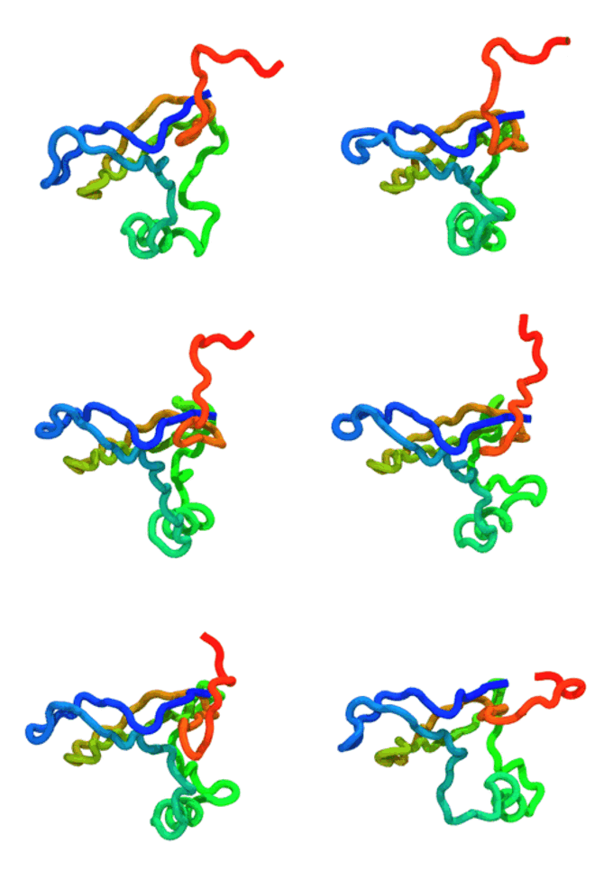
The run — 3 000-step Langevin dynamics at 300 K; the calibrated nscale keeps the fold stable. CA trace coloured N→C (blue→red).

The GIF is produced by tutorials/_viz/render_cg.py (headless VMD + Tachyon) after you run the tutorial — regenerate it any time with the command in step 5.

Files in this folder¶

File	Role
`P0CX28_clean.pdb`	Input structure (all-atom PDB; TOPO keeps only the CA atoms).
`domain.yaml`	Defines the single domain and its calibrated contact nscale.
`md.ini`	Simulation configuration (steps, temperature, I/O, hardware).
`run_simulation.py`	The runner script (reads `md.ini`, builds the model, runs MD).

Background concepts¶

Coarse-graining. TOPO reads your all-atom PDB but keeps one bead per residue at the alpha-carbon position. A 106-residue protein → 106 particles.
Structure-based force field. The native contacts in P0CX28_clean.pdb define the attractive interactions.
Contact nscale is a calibration parameter. Even for a single domain, domain.yaml carries a nscale — the global scale factor on the sidechain–sidechain contact energies. It is tuned so the model reproduces a target property (here, realistic stability at 300 K); for P0CX28 the calibrated value is 2.5044. The raw, unscaled value (1.0) would leave the protein under-stabilized and only marginally folded. Tutorial 2 generalizes this to different nscales per domain and across domain interfaces. For the full domain.yaml syntax — every key, its type, and the YAML basics — see Domain definition file.
STRIDE. On the first run TOPO calls stride on the PDB to find backbone hydrogen bonds and writes P0CX28_clean_stride.dat. You don’t manage this file by hand.

Want the full theory? The force field — bonds, the bimodal Gaussian angle, sequence-dependent periodic torsions, Debye–Hückel electrostatics, and the 12-10-6 structure-based contact potential — is documented term by term, with all constants and parameter sources, in The TOPO model: theory & force field.

Step-by-step¶

1. Check your environment¶

From this folder:

python -c "import topo, openmm; print('OK', openmm.__version__)"
which stride

Both must succeed (see the tutorials overview for setup).

2. Look at `md.ini`¶

Open md.ini. The important lines:

md_steps = 5000          # how long to run (short, for a demo)
ref_t = 300              # temperature in Kelvin
pbc = no                 # no periodic box (single protein, no solvent)
pdb_file = P0CX28_clean.pdb
domain_def = domain.yaml # single domain with the calibrated contact nscale (2.5044)
device = CPU             # runs anywhere; switch to GPU if you have CUDA
minimize = no            # native structure is already the energy minimum

There is no stride_output_file line, so STRIDE is run automatically (next step).

3. Run it¶

python run_simulation.py -f md.ini

You’ll see TOPO build the model (it prints the number of chains, adds each force term, runs STRIDE, builds the contact matrices) and then step the dynamics. It ends with --- Finished in … seconds ---.

4. Inspect the outputs¶

All generated files land in a single run folder, traj/ (created automatically), named traj.*:

File	What it is
`traj/traj.log`	Fixed-width, space-aligned energy/temperature log (one line every `nstlog` steps).
`traj/traj.dcd`	Trajectory (coordinates every `nstxout` steps) — open with VMD/MDAnalysis.
`traj/traj.chk`	Binary checkpoint (positions + velocities) for restarting (Tutorial 3).
`traj/traj.psf`	Topology of the CA model (for loading the DCD in analysis tools).
`traj/traj_final.pdb`	Last conformation (CA PDB); reuse as `init_position` to seed a follow-up run.
`traj/traj_runinfo.log`	Run provenance: package versions, hardware, GPU, timing.
`P0CX28_clean_stride.dat`	Cached STRIDE output (auto-generated, next to the input PDB).

Peek at the log:

head traj/traj.log

The columns are step, time (ps), potential / kinetic / total energy (kJ/mol), temperature (K), speed, and remaining time. A stable temperature near 300 K and a non-exploding potential energy mean the run is healthy.

5. Visualize (optional)¶

Regenerate the trajectory GIF at the top of this page straight from your run. Needs vmd and ImageMagick convert:

python ../_viz/render_cg.py --psf traj/traj.psf --dcd traj/traj.dcd --out img

The GIF animates every frame of traj.dcd; the CA chain is drawn as a smooth tube coloured N→C. See python ../_viz/render_cg.py -h for all options (width, stride, colour mode).

Try next¶

Bump md_steps to 50000 and watch the trajectory in VMD: vmd traj/traj.psf traj/traj.dcd.
Raise ref_t toward the protein’s unfolding temperature and look for the potential energy climbing as native contacts break.
Move on to Tutorial 2 to handle a multidomain protein.

Tip: each run overwrites the traj/ folder. To keep a run, copy the folder aside or point output_dir at a new folder (e.g. output_dir = runs/P0CX28_T300).