Tutorial 2 — Multidomain proteins & per-domain contact scaling
Goal: simulate a multidomain protein and control the contact-energy nscale
within each domain and across domain interfaces using a domain.yaml
file. We use adenylate kinase (1AKE chain A, 214 residues), a textbook
multidomain enzyme.
Time: ~4 seconds on a CPU.
Prerequisite: do Tutorial 1 first.
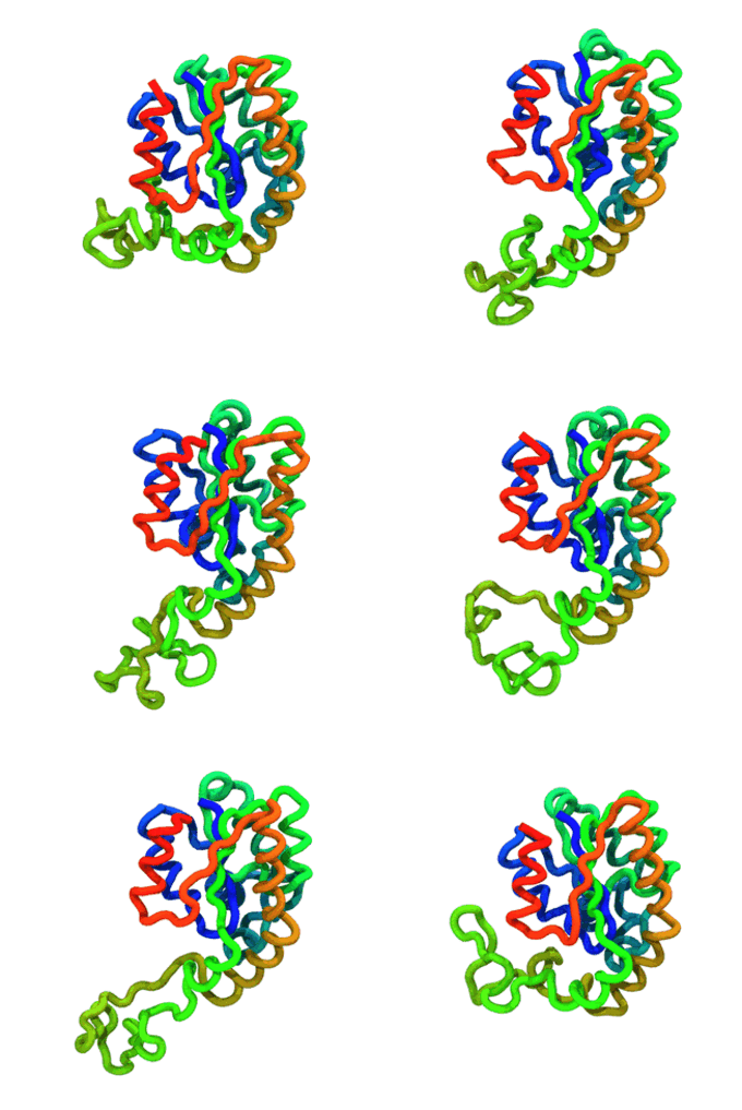
The run — Langevin dynamics at 300 K; per-domain and interface nscale keep both domains folded.
Regenerate after your run with
python ../_viz/render_cg.py --psf traj/traj.psf --dcd traj/traj.dcd --out img --hero 0 --stride 2.
Files in this folder
File |
Role |
|---|---|
|
Input structure (adenylate kinase, chain A). |
|
Domain definition — the new ingredient in this tutorial. |
|
Simulation config; note the added |
|
The runner script. |
Why domains matter
In a structure-based model, every native contact gets an attractive well. By
default all wells have the same relative nscale. But a multidomain protein
often needs different stabilities for each domain and for the interface
between them (e.g. to reproduce experimental melting temperatures, or to study
domain-wise unfolding). domain.yaml lets you set a scale factor on the
sidechain–sidechain contact energy:
within each domain (
intra_domains[...].nscale), andbetween domains (
inter_domains).
The key idea: discontiguous domains
Adenylate kinase’s CORE domain is not a single stretch of sequence. It is made of two segments — residues 1–117 and 166–214 — that fold together around the inserted NMP-binding domain (118–165). TOPO handles this by letting one domain list multiple residue ranges.
Open domain.yaml:
n_residues: 214
intra_domains:
  A:
    residues: [1-117, 166-214]   # ONE domain, TWO sequence segments
    nscale: 1.1556
  B:
    residues: [118-165]
    nscale: 1.6871
inter_domains:
  A-B: 1.8611
Reading it out:
Domain A = residues 1–117 and 166–214; all A–A native contacts (including contacts between the two segments) scaled by 1.1556.
Domain B = residues 118–165; B–B contacts scaled by 1.6871.
A–B interface contacts scaled by 1.8611.
Note: an unspecified interface defaults to scale 1.0 (native contacts kept, unscaled) — the scaling only modulates contacts that already exist in the structure. To intentionally decouple two domains, set their pair to
0.0explicitly. Full rules: Domain definition file.
Step-by-step
1. Note the one change in md.ini
Compared with Tutorial 1, the only addition is:
domain_def = domain.yaml
That single line switches on domain-aware contact scaling.
2. Run it
python run_simulation.py -f md.ini
In the build log you’ll see Domain definition file: domain.yaml, a
contact matrices: (214, 214) line and a native contacts: … | non-native pairs: …
summary, confirming the 214×214 contact matrices were built with your scaling applied.
3. Outputs
Same set as Tutorial 1, in the traj/ run folder:
traj/traj.log, traj/traj.dcd, traj/traj.chk, traj/traj.psf,
traj/traj_final.pdb, traj/traj_runinfo.log (plus the cached STRIDE
*_stride.dat next to the input PDB).
Build your own domain.yaml
Decide how many domains and which residues belong to each (a discontiguous domain just gets several ranges in its
residueslist).Set
n_residuesto the true residue count (must cover all residues; any residue you forget is auto-assigned to a fallback domainXwith nscale 1.0).Give every domain a numeric
nscale(a blank value errors).Add an
inter_domainsentry only for interfaces whose nscale you want to change from the default of 1.0 (set0.0to remove an interface; omitted pairs stay at 1.0).
The reference doc has six worked scenarios (single domain, contiguous, discontiguous, decoupled, 3+ domains, partial assignment): Domain definition file.
Try next
Make domain B much weaker (e.g.
nscale: 0.5), run, and watch B unfold first at elevated temperature while A stays folded.Set
inter_domains: A-B: 0.0to decouple the domains and observe them moving independently.Continue to Tutorial 3 to learn restarting and the output files in depth.